Galaxy Zoo

I would like spend a little time promoting the website known as Galaxy Zoo.  You can find it at www.galaxyzoo.org

Galaxy Zoo is this really neat way to get people to do science from their computers at home.  The idea is that Hubble and other telescopes produce too many images of galaxies for researchers to look at, and computers aren't very good at image recognition, so the researchers allow whoever wants to work on the project access to various images.  The researchers then have these people answer some simple questions that help define the characteristics of the galaxies.  The researchers can get thousands of answers for the same galaxy and then figure out which answer is the most likely to be accurate.  The people collecting data from Galaxy Zoo this are particularly interested in merging galaxies and sometimes you manage to find an image that contains two colliding galaxies!

When you first register for Galaxy Zoo, they'll put you through a straightforward tutorial and lure you in with awesome pictures like this spiral galaxy:

or this elliptical galaxy:

Once you log-in and start classifying galaxies, though, many of them will end up looking rather lumpy, kind of like this:

In spite of this initial false advertising, Galaxy Zoo is still a lot of fun and dangerously addicting.  I've already been distracted by it twice while writing this blog post.  If you feel guilty about procrastinating, this is a great way to put off your work without feeling bad, because it's still helping science progress.  It's probably even helping more than your latest physics set.  (Not that you needed any more motivation to procrastinate.)  Anyway, you occasionally do come across some really cool pictures.  They let you save any images that particularly grab your attention.  A few of my favorite galaxy images are below:

These are all images that I happened to find while classifying galaxies.  How does this whole classifying procedure work, I hear you asking?

The first thing you do is classify the galaxy as a smooth/elliptical galaxy, a spiral galaxy, or a star/artifact.  Galaxy Zoo then asks you about the shape if it's an elliptical galaxy and about tightness and number of spirals if it is a spiral galaxy.  They also ask about the presence of a bar and the prominence of the center bulge for spiral galaxies.  The last thing they ask about both types of galaxies is the most interesting:  Is there anything odd in the image?  If you pick yes for this question, then you get to specify what is so strange about this image.  Are there two merging galaxies?  Dust trails?  Is the galaxy irregular?  Perhaps most exciting is that you can specify lensing!  That's right, you can sometimes get images that show how galaxies can act as a gravitational lens!  It's quite rare, but if you see a star or another galaxy on one side of the main galaxy and then it appears again on the other side, the light coming from that object may be bending around the main galaxy and therefore the object looks like it's in multiple places!  Did I mention that I find this really cool?!  Unfortunately, I haven't come across any images of obvious gravitational lensing in any of the galaxies I've classified, but here is an example of an image in which somebody else on Galaxy Zoo found lensing:

The yellow blob is the galaxy and grey arc is the bent light from whatever object is behind the galaxy.  Isn't general relativity awesome?!  Perhaps I am getting overly excited...

If galaxies and their strange features aren't making you as excited as they are making me, then there are many other projects like Galaxy Zoo that have been created by Zooniverse. These projects all center on allowing the public try out a little science at home and letting humans pick up the slack where computers fall short.  So far, Zooniverse has projects for deciphering ancient Greek texts, examining the ice composition on Pluto and other objects on the edge of our solar system, looking for patterns that would indicate exoplanets in images from Kepler, looking for stellar nurseries in the Milky Way, examining features on the moon in images from the Lunar Reconnaissance Orbiter, and monitoring solar storms.  So before computers become good at pattern recognition in images, go to zooniverse.org and pick a project that catches your interest.  You never know when something really strange will pop up.  It might even lead to new science!

Black Body Radiation

Ay 20 – Set 4:  Black Body Radiation

Problem 2a

Primary author:  Joanna Robaszewski

Secondary author:  Cassi Lochhaas

Abstract

This problem demonstrates the relationship between the black body intensity 

and the black body intensity

by examining the units of each.

Introduction

A black body is something that emits radiation perfectly so that the properties of the emitted light are solely dependent on the temperature of the body.  The intensity of a black body is a measurement of energy per time, per frequency, per area.  We can use either the frequency ν or the wavelength λ to look at the intensity at some particular frequency.  So we get the equations:

Where h is 6.6 x 10^-27 erg*s and k is 1.4 x 10^-16 ergs K^-1 , T is the temperature of the black body, and c is the speed of light.

Questions and Results

2.a  We want to convert the units of the black body intensity from 

to

Let’s start by asking what are the units on B_nu?

Which simplifies to:

So to go from the units of B_nu to the units of B_lambda, what do we have to multiply B_nu  by?

We need to get another unit of centimeters in the denominator, along with seconds squared.

We know that frequency has units of s^-1 so we should try multiplying by the frequency squared.  If we do this we get the following units:

This is slightly closer to what we are looking for, but we still need centimeters cubed to end up in the denominator.

Let’s consider the relationship:

We want λ in terms of ν so if we solve for λ we get:

which has units of cm.  We want another factor of cm in the denominator, so if we take the reciprocal, we will get:

with units of cm^-1.

So if we multiply B_nu by:

which has units of:

we get:

which are the units of B_lambda!

And all we had to do was multiply 

 Here is a picture of a physicist's representation of a cow in space as a spherical black body.  Please note that the jet packs do not emit any radiation in this particular situation and there are no stars in the background because the exposure time was not very long.

Celestial Music vs. Sickly Orange Barf Glow

The other day we watched this time lapse http://www.youtube.com/watch?v=Rk6_hdRtJOE in class.  I've been watching it many times over since then and it's simply incredible.  I love watching the meteors go against the stars, I love how I gain the fleeting feeling that the Earth is a sphere, I love watching the clouds look like water.  I love watching the trees blow in the wind and watching the stars rise and set and knowing that this will continue for a long, long time.  And I love how it makes me marvel at the incomprehensibility of the size of the universe.  I know many people are not comfortable with the idea of being insignificant in the universe.  But can you imagine if our actions actually did have an impact on the universe as a whole?  How would we manage the courage to do anything at all?  As T. S. Eliot would ask in "The Love Song of J. Alfred Prufrock",  "Do I dare / Disturb the universe?"  I manage to find comfort in the fact that I can still help the people around me and make an impact in their lives, ideally a positive one, and in the fact that it is still possible to have an impact on a global scale, if you're lucky.  No, this is still not significant in the universe as a whole, but why shouldn't it be significant to us?

I sometimes feel guilty in my choice to go into science.  I know that without basic research we would not advance in technology and engineering and I know that complacency shouldn't be rewarded.  But sometimes I still feel like I should be doing something more practical, something that will help improve people's lives more directly.  Yet when I watch this time lapse, I feel a little better and I remember why I came to science in the first place.  How could I not wonder at our place in the universe after watching something like that?  How could I not be entranced and lured by science's beauty?  Seeing those images makes me want to understand nature so I can appreciate it better.  And I have not encountered anything better than science to accomplish that.  Maybe if we start to learn about the world around us, we will all appreciate it more and come to peace with our place in it.  I still haven't been able to completely shake the feeling that I should work on making other people's lives better, but I also know that science is a noble and worthwhile pursuit, one that I will not give up on very easily.

Not everything in the video was uplifting, though.  In the final time lapse in the video, it is hard not to focus on how much of the night sky is being taken over by light from the ground.  I was once walking under the orange clouds that are the Los Angles night sky and remembered a quote from The Simpsons.  In this particular episode, Lisa has become interested in astronomy and despairs at the fact that she can't see anything through her telescope due to light pollution.  She remarks that "nobody ever wrote a poem about sickly orange barf glow" and she'd rather see the stars.  I took that as a challenge and wrote a poem about the sickly orange barf glow of the L.A. sky.  (Well, it's actually more of a song.  You can sing it to the tune of the Winnie the Pooh Little Black Rain Cloud song, if you desire.)  Here are the lyrics:

I'm just sickly orange barf glow
Hanging over L.A.,
Taking your night sky away.
Everybody knows that smog clouds
Send acid rain down.
I'm just hovering around,
Over the ground,
Making astronomers frown.

So there's a poem about sickly orange barf glow.  But I'd still rather have stars.

Hot Flares from Cool Stars

The Catalina Sky Survey (CSS) is a synoptic survey that scans the entire sky repeatedly and gathers information on various objects.  CSS focuses on near-Earth asteroids, which leaves a lot of other data for other researchers to take a look at.  The Catalina Real-Time Transient Survey (CRTS) is a survey that uses some of the left over CSS data.  What CRTS is mapping and studying are transient objects, these are objects that vary in brightness over time.  Transient objects include supernovae, blazars, and flare stars.

Through Caltech's summer undergraduate research fellowship (SURF) program, I spent the last summer studying the flare stars in CRTS data.  Flare stars are a particularly interesting type of star because they are often younger, smaller, and cooler than the sun, but they produce enormous stellar flares that are much larger than solar flares.  It is thought that the stellar flares are caused by the same mechanism that causes solar flares.  This mechanism involves the magnetic fields around a star shifting until they align in such a way that the star's plasma is suddenly accelerated in a large plume or arc.  You can imagine something like the solar flare seen in this image from NASA:

The stellar flares only last for a few minutes, but can increase the star's brightness by an order of magnitude!  Below, I have some images from CRTS that captured a flare star while it was flaring:

In the image on the left the star is not flaring, whereas in the image on the right, the increase in magnitude implies the star is undergoing a stellar flare.  These images are from the Catalina Real-Time Transient Survey database.

CRTS has tens of thousands of light curves just for flare stars alone.  When you add that to the other thousands of objects it has observed it becomes difficult to classify the light curves by hand.  The goal of my project was to come up with an efficient way of sorting out the flare star light curves from the non-flare star light curves.  Later, we wanted to examine the flare star light curves to define common characteristics of flare stars and look for correlations with spectral type to help classify flare stars for future synoptic surveys.  If we could do that then we would understand the nature of flare stars better and other surveys could be more efficient in their searches.  If the surveys were interested in flare stars then they would know what to look for, and if they were interested in a different phenomenon then they could stop spending time on objects that were likely to be flare stars.

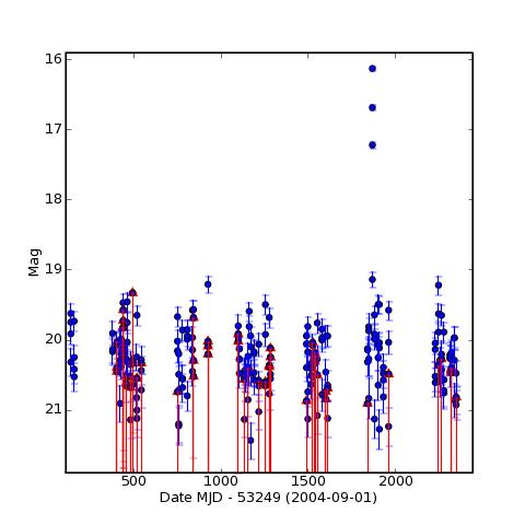
The sort of light curves we were dealing with looked like this:

If you don't have an astronomy background, the way light curves work is time is on the x-axis, as measured by the Modified Julian date (MJD is just a calendar astronomers use, it counts the days since a particular time) and magnitude is on the y-axis.  The magnitude axis looks like it is upside down, but the way magnitude is measured means that a larger number indicates a dimmer star.  So brighter stars go closer to the top of the plot.  In this plot, there is only one star and each point is a different observation of that star.  We can see that there are three points that are much higher than all the rest.  These are from the observations that were made when the star was flaring.  The flares are typically a few minutes long, so we would expect to see the flaring observations all stacked on top of each other, plotted on the same night.  This light curve is also from the Catalina Real-Time Transient Survey database.

Light curves from other objects would look different.  For example, a supernova would get bright very quickly and then slowly decay over the course of a few days, depending on the type of supernova.  We wouldn't expect to see such a drastic decrease in magnitude in a supernova light curve.  Since different transient objects produce different patterns in their light curves, we can exploit this to write a program to notice these differences and classify the light curves.

One requirement we might pick for the program to classify the light curve as a flare star is that the light curves shows at least one point that is significantly higher in magnitude than the average magnitude.  We can set a value for what qualifies as "significantly higher" but this may need to be changed later if we find out that many flare stars produce short flares, flares with smaller amplitudes than expected, and we have been discarding them since they didn't meet our requirement.  We may also need to change this value if it is too small and we have been acquiring many false positives.  To figure out if we need to change this value, we can test the program on light curves that have already been classified and see if it is giving reasonable results.  But even if the program is doing well, we still may need to change it if new science comes in about the short flares that I previously mentioned.

We should also probably specify how many of these observations should have high magnitudes.  We don't want too much of the light curve to be high.  I ended up putting the limit at 10% of the observations.  We also don't want too few of the points to be high, because then the program may classify a light curve based on an outlier.  So let's specify that there have to be at least four observations on any given night and at least three of the four observations need to be above the average magnitude by at least the value that we picked earlier.

Flare stars are also not periodic.  This means that if we spot multiple observations that are high enough to qualify as flares, but on different nights, the light curve we are looking at probably does not belong to a flare star.  If the high magnitude observations were spread out over multiple nights, the likelihood that the object in question is something like a supernova increases.

Once we can code all these criteria in to a program, we can run the program on the light curves that have not been classified.  If the program finds a light curve that meets all the specified requirements, it will write the name of the object associated with the light curve in a list and label it a flare star.  Otherwise the object is labeled as a non-flare star.  How to classify those remaining objects is up to the next person to work on this project.

After we get a list of our objects with the classifications back, we should check if the results are reasonable.  We can do this by plotting some the light curves that were classified as flare stars.  If there is some reason why the program classified light curves as flare stars when they obviously do not meet the criteria, there may be something wrong with the code or our assumptions about what qualifies as a flare star.  If there is no consistent reason why light curves were incorrectly classified, we can look in the Sloan Digital Sky Survey database to see if there are any optical artifacts or nearby stars that may be interfering with the observations.  Finally, we can also check the spectra associated with the object to see if it matches that of a typical young, red flare star.  Or we could get our own spectra for interesting candidates!  But that's a story for another day.

Once we check the accuracy of the program, and it is doing well, we can start extracting data from the light curves that will help us classify flare stars for CRTS and other surveys.  Unfortunately, I ran out of time before I could get to that part of the project.  So if anybody is interested in working on something like that, you should talk to Professor Djorgovski.  He was a really good mentor to work with over the summer.  Good luck!

Follow up on LST

A recent alum was reading my post on local sidereal time and mentioned something rather cool.  Apparently, the constellation Cassiopeia, the constellation that looks like this:

 

has a right ascension of about 0 hours.  For those of you without an astronomy background, right ascension is one of the coordinates astronomers use to describe the position of the stars.  It is sort of like longitude, except it measures how far east a star is in comparison to where the sun is during the vernal equinox instead of using the Prime Meridian.  Since local sidereal time describes which right ascension is overhead at a specific time, we know that when Cassiopeia is directly overhead and forming an 'M' the LST is 00:00.  When Cassiopeia is a 'W' the LST is 12:00.  When Cassiopeia is directly left of Polaris (the North star), the LST is 6:00 and when it is to the right of Polaris, the LST is 18:00.  So if you're ever walking around at night and wondering if an object with a certain right ascension will be visible (and the declination isn't an issue) and you can find Cassiopeia, then you may be able to tell how close to your meridian the object you are looking for is.

Thanks to http://stargazer2010.files.wordpress.com for the picture and Joe A. for the information.

Measuring the Earth's Radius

Ay 20 – Lab 1:  The Radius of the Earth

By:  Joanna Robaszewski

Purpose of experiment:  To determine the Earth’s radius by using only a stop watch and a clear view of the sun as it sets

Procedure:  We drove to Santa Monica beach on September 30, 2011 and arrived approximately at 6:15 pm.  The sun was supposed to set at 6:40 pm.  Some students lay on the sand while my group stood on the balcony surrounding the lifeguard house.  There were also some students of the pier.  The set-up is shown below: 

We had planned on taking two measurements with the stop watches.  First, the observers on the ground would signal to us standing on the lifeguard balcony when the bottom rim of the sun was tangent with the horizon by waving their arms.  We would then start the stop watches.  We were supposed to stop the stop watches when the bottom edge of the sun hit the horizon from our perspective on the lifeguard balcony.  This first measurement was not completed, however, because to us on the balcony it looked like the bottom of the sun had already touched the horizon before the observers on the ground signaled to us.  We were able to complete the second measurement.  This measurement consisted of starting the stop watches when the observers on the ground signaled that the top edge of the sun had touched the horizon by waving their arms and then stopping the watches when it appeared to us that the top edge had touched the horizon.

Data/Results:  The time measured by the stop watches between when the people on the ground saw the top of the sun set and when those of us on the lifeguard balcony saw the top of the sun set was 4.05 seconds.  We estimated the height of the balcony to be 5 feet.  I am 5’8”.  The total height from the ground was then 10’8” = 3.25 meters.  Looking at the Earth from the side we see:

We know that it takes approximately 24 hours for the Earth to rotate 360°.  How many seconds does it take?

So in the 4.05 seconds we measured, the Earth rotated:

This should be equivalent to θ in the diagram showing Earth from a side view.

We can then find the value of the longer leg of the triangle:

(I apologize that the diagram is slightly blurry, the short leg of the triangle reads "h = 3.25m")

Since x is such a small fraction of the Earth’s circumference, it can be approximated as straight.  The law of sines can then be applied:

Now that x is known, r can be found using the relation:

The Earth fact sheet from the NASA website (nssdc.gsfc.nasa.gov/planetary/factsheet/earthfact.html) gives the Earth’s radius as 6371 km.  So the accepted value for the Earth’s radius, R, is:

Error Analysis:  According to www.humanbenchmark.com/tests/reactiontime/stats.php the average reaction time to click on a target is 200 ms = .2 s.  We will take this as the reaction time for the people on the ground to wave as they saw the top of the sun set, as the reaction time for us to see the waving and press start, and as the time for us to press stop as we saw the top of the sun set.  The first action and reaction (seeing and waving) would have decreased the time measured, as would the time taken between waving and pressing start.  The time to press stop, however, would have increased the time, so let’s say that the uncertainty on the time measurement was .2 seconds.  In that case the time measured was:

Since we estimated the height of the balcony by comparing it to the height of a person with a known height rather than measuring it with a more precise tool such as a meter stick, the uncertainty in the height is:

To find the uncertainty of our result for the Earth’s radius we need to propagate error:

We know

from:

and we know

from law of sines.  

I apologize for the algebra in advance…

Relating these gives:

Substituting t = 4.05s and simplifying gives:

Remembering that:

Substituting the values calculated and estimated earlier gives:

So our calculated result for the Earth’s radius was:

(Hooray, the uncertainty is smaller than the result!)

To find how many standard deviations our result is from the accepted value:

Our result is within 16 standard deviations of the accepted value.  This comparison is rather poor.  Sources of error when calculating the radius of the Earth may have come from underestimating the reaction times, not having many data points to average out errors, atmospheric and smog interference, and any assumptions about parts of the Earth’s circumference being straight.

Follow-up - Mass of the Earth:  Using our value for the radius of the Earth we want to calculate the mass of the Earth.  We can use the relation:

The density of the Earth can be approximated by the density of the average rock.  Most rocks sink, but some float in water.  So let’s say the density is between 1 and 10 times that of water.  Let’s take an average of the two and approximate the density of the average rock, and the Earth, as 5000 kg/m^3.

In that case:

and the uncertainty is:

So our value for the Earth’s mass is:

The accepted value for Earth’s mass is 5.9736*10^24 kg, as given by the same source used to find the Earth’s radius, NASA’s planetary facts sheet.

Our value of the Earth’s mass is within:

of the accepted value for the Earth’s mass.  This comparison is also poor.  The value found for the Earth’s radius was also far from the accepted value and the error was propagated, so all the sources of error described in the previous section still hold.  Additionally, the density of the Earth was only an approximation and that would add to the error as well.